Combining Harmonic Motions in One Dimension
We saw, in the previous section, that the solution to a second degree linear equation in one dimension of the form
| d 2x | = | |
| - ωo2 x | ||
| dt 2 |
can be expressed in a number of ways.
We also mentioned that where a system is linear, its displacement at any time is found by adding together the individual displacements due to each harmonic motion.
Let us consider a system moving under the influence of movement described by two expressions with a common frequency, ω
x 1 = A 1 exp j ( ω t + φ 1 ) , and
x 2 = A 2 exp j ( ω t + φ 2 ) .
x 1 and x 1 are complex.
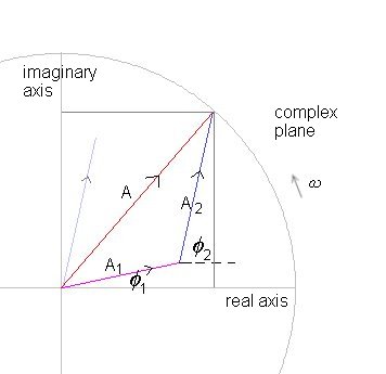
We have shown these in the diagram below as two phasors, each rotating, in the complex plane in an anti-clockwise direction with angular velocity ω
The pale blue and purple lines are the position phasors as they would be represented individually. To add two phasors, one places the tail of one phasor A2 at the head of the other phasor A1. The resultant phasor is the line A. The resultant can be found too by placing the tail of A1 at the head of the other phasor A2. The order of the addition is immaterial. The length of A A is the resultant amplitude while the angle it makes with the real axis is the resultant phase angle φ .
The expression for the resultant is a simple harmonic vibration with the same frequency as the original harmonic vibrations.
x 1 + x 2 = A 1 exp j ( ω t + φ 1 ) + A 2 exp j ( ω t + φ 2 ) , or
x = A exp j ( ω t + φ ) , where
| A = |
|
|
| ( A 1 cos φ 1 + A 2 cos φ 2 ) 2 + ( A 1 sin φ 1 + A 2 sin φ 2 ) 2 |
and
| tan φ = | A 1 sin φ 1 + A 2 sin φ 2 A 1 cos φ 1 + A 2 cos φ 2 |
This solution can generalized where there are many harmonic vibrations all with the same frequency. In that case the amplitude and phase angle are
| A = |
|
|
| ( Σ A i cos φ i ) 2 + (Σ A i sin φ i) 2 |
and
| tan φ = | Σ A i sin φ i Σ A i cos φ i |
The real displacement is, of course, the projection of the complex variable x onto the real axis which is the sum of the projection of each x n.
Where the harmonic motions have different frequencies the analysis is similar.
x 1 = A 1 exp j ( ω 1 t + φ 1 ) , and
x 2 = A 2 exp j ( ω 2 t + φ 2 ) so that
x 1 + x 2 = A 1 exp j ( ω 1 t + φ 1 ) + A 2 exp j ( ω 2 t + φ 2 ).
We introduce the term Δ ω = ω 2 - ω 1 so that we can now write the linear superposition in the form
x = A 1 exp j ( ω 1 t + φ 1 ) + A 2 exp j ( ω 1 t + Δ ω t + φ 2 )
Inspection of the solution indicates that both the amplitude A and the phase φ vary with time, in other words, they are not constants. The time dependence of the amplitude produces 'beating', in which the listener hears a slower modulation particularly if the 'beat' frequency is small (no much greater than ten cycles per seond) which can be the case when the frequencies of the original harmonic motions are almost identical.
The final solution can be written as
x = A (t) exp j ( ω 1 t + φ (t) ) , where
| A (t) = |
|
|
| A 1 2 + A 2 2 + 2 A 1 A 2 cos ( φ 1 - φ 2 - Δ ω t ) |
and
| tan φ (t) = | A 1 sin φ 1 + A 2 sin ( φ 2 + Δ ω t ) A 1 cos φ 1 + A 2 cos ( φ 2 + Δ ω t ) |
We illustrate the result in the diagram below
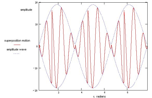
The linear superposition generally results in non-simple 'harmonic' motion, shown in red.
The lower frequency, quasi-simple harmonic wave shown as a dotted blue line is a periodic amplitude wave that, when of low enough frequency, will be perceived as a 'beat'. In the general case the amplitude varies between ( A 1 + A 2 ) and ( A 1 - A 2 ) .
In situations where the original waves have identical phases and identical amplitudes the frequencies are almost identical, the beats would be particularly audible and the amplitude would vary periodically between twice the original amplitude and zero. These results can be shown by making the required substitutions A 1 = A 2 and φ 1 = φ 2 in the equations for A (t) and φ (t) that we have derived above.
In this case we may conclude that from two waves with identical phase and amplitude but frequencies ω 1 and ω 2 we will produce a resultant wave of average frequency ( ω 1 + ω 2 ) / 2 and amplitude varying with a frequency given by ( ω 1 - ω 2 )
The illustration above is of motion that is not simple harmonic and which is not associated with a particular frequency. And yet, we originated the expression that describes this complicated motion from the sum of simple harmonic waves, waves that could be expressed as cosine functions that are themselves the solutions to linear differential equations whose properties are time independent. This points us to a powerful way of handling complicated motion. All we need to do is find a way of expressing any motion as the sum of cosine functions each with a suitable choice of amplitude and phase. Each cosine function represents a particular 'mode'. So we find that any linear vibrating system is equivalent to a set of independent harmonic oscillators with natural frequencies corresponding to these modes. Further more, the case where we have two motions with different frequencies, which we considered above, is actually the same as we considered in the previous section when discussing the transient behaviour of forced oscillations of a system subject to damping. Our case above is of two persistant waves that effectively move between a number of quasi-steady states which over time oscillate between two extremes. We have plotted the states in terms of amplitude but we know that the square of the amplitude is the energy so that we are, effectively, observing changes in energy when we see changes in amplitude. In the case of the initially transient behaviour of a damped free oscillator subject to an external force, the transient behaviour cannot persist. In the end, the system must find a unique solution that reflects the persistent driving force. |
Combining Harmonic Motions in Two Dimensions
This section is currently under construction - more material will be added shortly.
