Periodicity, Frequency and Amplitude
"Anyone who wants to analyze the properties of matter in a real problem might want to start by writing down the fundamental equations and then try to solve them mathematically. Although there are people who try to use such an approach these people are the failures in this field; the real successes come to those who start from a physical point of view, people who have a rough idea where they are going and then begin by making the right kind of approximations, knowing what is big and what is small in a given complicated situation. These problems are so complicated that even an elementary understanding, though inaccurate and incomplete, is worth while having, and so the subject will be one that we shall go over again and again, each time with more and more accuracy, as we go through our course in physics." from The Feynman Lectures on Physics Volume 1 section 39-1
A musical note is characterised by three properties; pitch (how high or low the note is), volume (how loud or soft), and its 'colour' or 'timbre'. If the note does not change pitch, we say it has a particular frequency (expressed in cycles per second or hertz, the scientific unit of frequency). The note we hear has a characteristic frequency, most commonly the fundamental frequency of the system from which the note eminates. The 'colour' or 'timbre' of a note is determined by a number of higher frequencies, sounding at the same time as the fundamental. When heard in combination, they give the note its 'colour'. This is why it is possible to distinguish the same note produced on different musical instruments. In some cases the higher frequencies are harmonics of the fundamental that are characteristic of the generating system. The harmonics associated with a vibrating string are one example. In other cases, the higher frequencies may be associated with a secondary process only weakly coupled to the primary resonator. The chiff from certain organ pipes would be a good example.
We will consider 'timbre' later. For the moment, we examine vibrations and frequency in a more general way.
We will consider the simple pendulum in some detail because of its historical importance. Other systems, that exhibit similar behaviour, we discuss towards the end of this section.
Free Oscillations - The Simple Pendulum
Galileo's study of the simple pendulum introduces us, as it introduced the modern scientific world, to a simple mechanical oscillator with a characteristic frequency. Because frequency is the reciprocal of the period, the system is said to be periodic or to have a characteristic periodicity. Crudely put, 'frequency' is the number of times a particular event occurs within a given time interval, while 'period' is the time interval between each of those events. It was the periodicity that struck Galileo as interesting and begged the question, why?
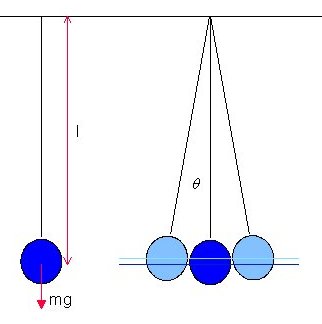
For our mathematical discussion, we 'idealise' the pendulum (see illustration above). It is a spherical weighted bob attached to one end of an inextensible, massless string, whose other end is fixed to a point on the ceiling. We are viewing the pendulum normal to the plane of motion. By making the bob spherical and the string massless, the centre of gravity of the bob is the centre of gravity of the whole pendulum. By making the string inextensible we know that the energy in the system is described only by the motion and position of the bob. When not in motion, the bob hangs directly below the fixed point of attachment (see left-hand illustration above). We ignore any resistance to the bob's motion from the air through which it moves.
In our diagram above, the two light blue bobs and strings (on the right), represent (i) the position from which the bob is released, and (ii) the position to which the pendulum swings after release. It is immaterial whether it is released from the right or from the left. The period is the time the bob takes to travel from the release point and back again. We have also marked two blue lines; the lower dark blue line marks the centre of gravity of the hanging resting bob (the lowest point the centre of gravity of the bob reaches during its motion) while the upper light blue line marks the centre of gravity of the bob at the moment of release and again when it is half way through a period of swing (which is the same height as the centre of gravity of the bob was when it is released).
We have indicated the weight of the bob (the product of its mass, m, and the acceleration due to gravity, g), the distance from the upper fixed point to the centre of gravity of the bob, l, and the angle the string makes when the bob is drawn to one side and released. This we denote θ. The total angle of swing is 2θ.
When the bob is drawn to one side and released, we notice a number of things about the way the bob swings. At the moment of release the bob is not moving, but it quickly picks up speed until it reaches the lowest point of its swing, after which it slows its speed until, reaching the point that is the reflection of the point of release in the vertical through the point where the string is attached to the ceiling, the bob finally comes, momentarily, to a stop. It then reverses its direction of motion and moves back towards the point of release.
From the observation that an object released a distance above the ground falls towards it, we can conclude that the motion of the bob is basically the same effect but the bob is constrained, by the string, to move in an arc rather than in a straight line towards the ground below. The centre of gravity of the bob is similarly constrained to move between the dark and light horizontal blue lines.
The dynamic behaviour of objects in free-fall gives us a clue as to how we might analyse the dynamics of our pendulum. When objects fall under gravity they accelerate. The longer they fall and the further they fall, the faster they travel. Isaac Newton, who first understood how bodies move under gravity, incorporated the work of Galileo and others into three Laws of Motion:
It is from arguments originally advanced by Galileo that we believe 'physical' laws to be 'universal'. They are 'true' for any set of objects, for any set of forces that might act on those objects, wherever one might choose to observe them and for any moment in time. We call this 'space-time invariance'. Because we understand physical quantities in terms of how they can be quantified (by their operational definition) we can design an experiment whose outcome can confirm or refute our beliefs. This position is the essence of 'logical positivism', sometimes also called 'logical empiricism', which matured in the Vienna of the 1920s and 30s and has been a dominant influence on twentieth century philosophical thought. We now know that Newton's Theory of Gravitation is erroneous. Hermann Minkowski, Henri Poincaré and Albert Einstein, by considering more deeply how time and distance are measured in inertial frames (by examining the 'operational definition' of time and space), showed that time and space are interconnected and that 'simultaneity' is 'relative'. In his famous 1908 lecture at the University of Göttingen, Minkowski announced: "Henceforth space by itself, and time by itself are doomed to fade away into mere shadows, and only a kind of union of the two will preserve an independent reality." For the systems we examine here, the Galilean-Newtonian theory is 'operationally' adequate. It gives us uncomplicated equations which we can manipulate, and its predictions are indistinguishable from our observations. However, from this definition of physical quantities and, by extension, the 'laws' that define their association, we come to appreciate Weizsäcker's comment that "Science is easier to practice than to understand". We should also avoid making the assumption that because we are apply the 'mathematical' techniques of the infinitesimal calculus, to 'mathematical' functions and equations, these techniques necessarily have any 'physical' significance. Their 'mathematical' soundness is no longer an issue, but modern physics has shown us that mass, energy, angular momentum, even time, are 'grainy'. We can no longer cling to the concept of a 'physical continuum'. |
Let us now look at the forces acting on the bob in greater detail.
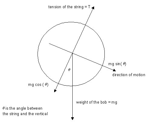
All forces act through the centre of gravity of the bob. The vertical downward force is that due to gravity acting on the mass of the bob. The bob is released when the string is at an angle θ to the vertical. The tension in the string, T, acts to constrain the centre of gravity of the bob to movement in the arc of a circle centred on the point of attachment on the ceiling. Because it acts perpendicularly to the direction of motion, it cannot accelerate the bob along its path.
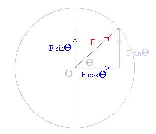
Replacing a single force with two forces acting at right angles to one another is called 'resolving the force'. If the original force (shown in red) is F and one resolved force is in a direction angle θ to the original force, then the resolved forces (shown in dark blue) will be F cos (θ) and F sin (θ).
The resolved forces act through the same point O as the original force and they should be thought of as the projections of the original force F on the orthogonal axes, two axes at right-angles to each other. One can show that the two forces are equivalent to the original force by comparing the magnitude and direction of the original force with that of the two 'resolved' forces. The square of the 'unresolved' force should equal the sum of the squares of the two 'resolved' forces. This follows from Pythagoras' theorem. F 2 cos 2 (θ) + F 2 sin 2 (θ) = F 2 [ cos 2 (θ) + sin 2 (θ) ] = F 2 The tangent of the angle between F and the resolved force F cos (θ) is the ratio of the two resolved forces
Using vector addition, where the tail of the vertical resolved force vector (shown pale blue) is placed at the head of the horizontal force vector, the equivalence is immediately clear. Treated as vectors, both the dark blue and the pale blue vertical forces are equivalent; both have identical magnitude and direction. |
We 'resolve' the forces in two perpendicular directions and use Newton's second law of motion in each direction. The tension in the string acts only perpendicularly to the path. The downward force due to gravity must be resolved into two forces, one acting in a direction perpendicular to the path, and the other acting in a direction parallel to the path. Any net force will be associated with acceleration in that direction.
perpendicular to the path:
T - mg cos (θ) | = | mv 2 l |
(the term on the right is the product of the mass of the bob m and the centripetal acceleration, the square of the speed v divided by the radius l).
parallel to the path:
- mg sin (θ) = ma
where a is the acceleration along the path. Note the minus sign in the second equation. As the angle between the string and the vertical increases the bob is slowed. The force retards the motion.
If we call the lateral displacement x, and assume that x is much smaller than l, then
| = | x | |
| sin (θ) | ||
| l |
We can now write the linear differential equation that describes the motion of our pendulum.
= | d 2x | = | gx | |
| a | ||||
| dt 2 | l |
The linear differential equation has constant coefficients and has a general solution of the form:
x = A cos (ωot) + B sin (ωot)
g | |
where A and B are constants to be determined by our initial conditions and ωo2 = | |
| l |
Alternatively, the solution may be expressed in a simpler form:
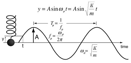
x = A cos (ωot + φ).
where A is the amplitude, ωo is the natural angular frequency of the system and φ is the initial phase of motion. Note that we have not changed the number of arbitrary constants. In the first solution the constants are A and B while in the second solution the two constants are A and φ. In both cases, the value of these arbitrary constants is determined by the initial conditions (for example: how far the bob is displaced before release) and not by the characteristics of the system itself (for example: mass of the bob or the length of the pendulum).
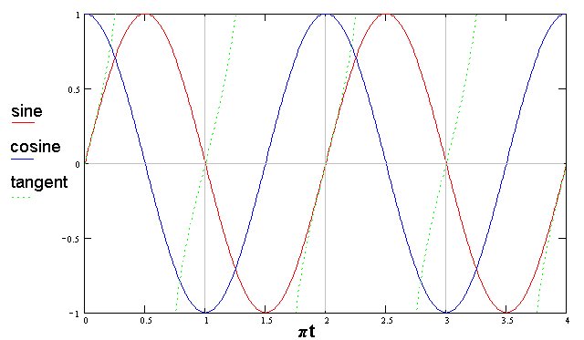
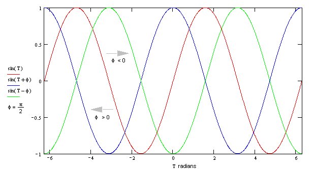
Trigonometric functions of which sine and cosine functions are but two, are periodic functions. We plot the three most common functions below. The horizontal axis shows the value of the argument t in units of π while the vertical axis shows the value of the function. When t = 0 the sine and tangent functions have the value zero, while the cosine function has the value +1.
The maximum value of the sine and cosine functions is +1. The minimum value is -1. If these functions are multiplied by a constant A , called the amplitude, the functions oscillate between + A and - A . The distance between successive maxima, or successive minima, is the period of the function. If the function is of the form sin ( t ), and the value t max returns the maximum value of the function then any value t max + 2 n π where n is an integer will also be a maximum. This is true for both sine and cosine functions. We show below the sine function with different values for the initial phase φ
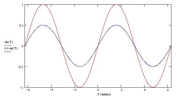
We show below the sine function with different amplitudes A.
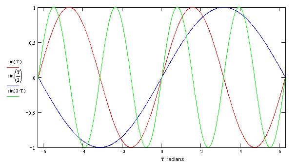
We show below the sine function with different frequencies ω o.
|
The amplitude for the simple pendulum is the maximum lateral displacement of the bob from its position when the pendulum is at rest. Because cos (ωot + φ) takes values between 1 and -1, we find that x, the position of the pendulum, takes positive values on one side of the equilibrium line and negative values on the other and the equilibrium line intersects the line of lateral displacement where x = 0.
The periodicity of this solution arises from the fact that cos (ωot + φ) = cos (ωot + φ + 2π), which reduces to
ωot1 = 2π + ωot2.
T o, the period, is given by the equation
2π | |
| T o = t1 - t2 = | |
| ωo |
ωo | 1 | ||
The natural frequency fo = | = | ||
| 2π | T o |
therefore
| = | 1 | g | ||
| fo | ||||
| 2π | l |
Linear differential equations with constant coefficients consist of a sum of terms, each term a derivative of the dependent variable (in this case x) with respect to the independent variable (in this case t) multiplied by a constant. A linear differential equation of order n, where the degree of an equation is the degree of the highest differential coefficient when the equation has been made rational and integral as far as the differential coefficients are concerned, would be of the general form:
An alternative notation (which we use below when discussing the energy equation) is: a n x n + a n-1 x n-1 + . . . . . + a 1 x 1 + a 0 x = f (t) Every term a i is a constant. An important property of the solutions to linear differential equations is that if a solution is multiplied by a constant, that new solution also satisfies the original differential equation. |
Linear Differential Equations with Complex Variables
The general solution of our linear differential equation can be solved using exponential functions and complex variables. If the solution contains only zeroth and first powers of x, it can be separated into its real and imaginary parts. The real part of the solution must satisfy the real part of the original linear differential equation and the imaginary part must satisfy the imaginary part of the original differential equation. Indeed, the real parts of the complex variables will then be the values of amplitude, frequency, position, motion, amplitude and so forth we found earlier. In certain circumstances, it is easier to manipulate the solution expressed this way than when it is written in terms of sine and cosine functions. However, the solutions are equivalent because, from Euler's Formula,
exp ( j ωot) = cos (ωot) + j sin (ωot)
and
exp ( -j ωot) = cos (ωot) - j sin (ωot)
where j is the square root of -1
x = A cos (ωot + φ) = Re[ A exp ( j ωot + j φ) ] = Re[ A exp ( j φ) exp ( j ωot) ]
where Re[] means 'take only the real part of the complex variable'. The complex variables displacement, velocity and acceleration may be thought of as vectors rotating in the complex plane (called 'phasors') with real angular velocity ωo. The real time dependence of each may be found by taking the projection of the complex quantity on the real axis (i.e. Re[]).
There is a fourth form of the solution where ωo is a complex number. In this case the solution may be written:
x = C exp ( j φ) exp ( j ωot ) + [ C exp ( j φ) exp ( j ωot ) ]*
where the second term, the expression within [ ]*, is the complex conjugate of the first term. The sum of a number and its complex conjugate is twice the real part of the number. Therefore, x is real, but we still have two unknowns, C and φ.
'Live' Demonstration of Simple Harmonic Motion
The behaviour of solutions of the differential equation associated with simple harmonic motion (SHM), is easier to understand by relating SHM to circular motion. This relationship is elegantly demonstrated on Professor Fu-Kwun Hwang's web site with a 'live' graphical demonstration.
The Energy Equation
Let us return to our differential equations in its most general form.
| = | d 2y | = | f (y) | |
| y2 | ||||
| dt 2 |
Writing the equation y2 = f (y) and multiplying each side by 2y1, where y1 = dy / dt, we get
2 y1 y2 = 2 f (y) y1
Integrating, with respect to t,
| = | dy | = | ||||||||
| y12 | 2 | f (y) | dt | 2 | f (y) dy | |||||
| dt |
This is the general form of the energy equation.
Taking the differential equation we met earlier
| d 2x | = | |
| - ωo2 x | ||
| dt 2 |
and using the method outlined above,
| 2 | dx dt 2 --- --- dt dx 2 | = | - 2 ωo2 x | dx --- dt |
Integrating with respect to t,
(dx / dt) 2 = ωo2 (a 2 - x 2)
where a is a constant of integration
(dx / dt) 2 = v 2
from which we find that the velocity is zero when x = a or x = - a.
For the simple pendulum these are the points of release and of momentary rest half way through the period of the swing.
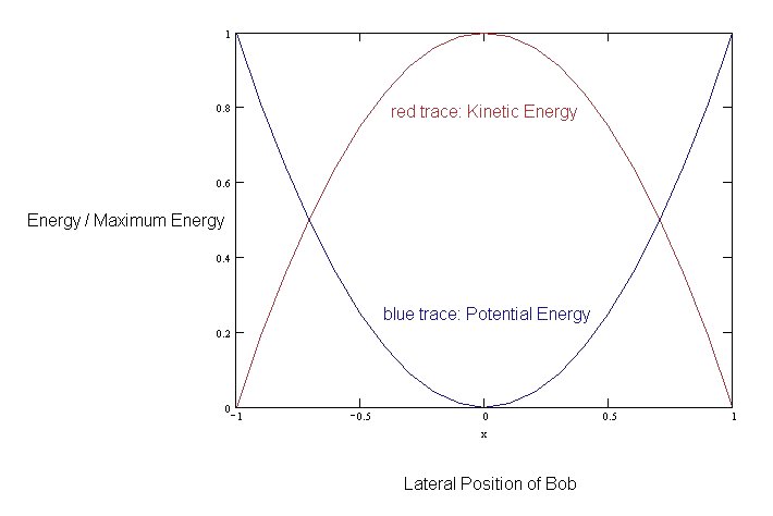
The maximum velocity of the bob occurs when x = 0 which is the lowest point on the arc of swing. Here the kinetic energy of the bob is at its maximum.
The general expression for the kinetic energy of the bob is mv 2 / 2. Its maximum value is m(ωoa) 2 / 2.
From the principle of the conservation of energy, the potential energy is the maximum energy less the kinetic energy.
m(ωoa) 2 / 2 - mv 2 / 2 = m(ωox) 2 / 2
The difference in potential energy of the bob when it is released and when it passes through the lowest point of the swing is the energy available for convertion into kinetic energy. Since the total energy (the sum of the potential energy and the kinetic energy) is constant during the period of the swing (because we have assumed that there is no loss of energy to the surrounding air due to air resistance) it is clear that it is also proportional to a 2, the square of the amplitude.
The energy equation may be used to find the relationship between position and time.
The solution is:
x = a cos (ωot + φ)
which is the result we found earlier, and where ωo can be the positive or negative root of ωo2.
We have been examining second order differential equations with one degree of freedom, denoted by x. It is possible to show analytically that where such a system remains close to equilibrium, equilibrium being where the potential energy is stationary (d (P.E.) / dt = 0), the behaviour will always be strictly harmonic and the period (and therefore the frequency) will depend only on the structure of the system (i.e. terms denoting 'inertia' and 'stiffness of an equivalent spring'). The amplitude and phase, however, will depend on external circumstances (i.e. on the initial conditions). This physical insight explains why, for the majority of musical instruments heard under normal playing conditions, volume (associated with the square of the amplitude) and pitch (associated with frequency) can be treated independently. |
Free Oscillations - Mass on a Spring
The motion of a mass m attached to a massless spring whose spring constant (sometimes called 'stiffness') is K, which moves vertically about its equilibrium position, exhibits simple harmonic motion, where ωo2 = (K / m). This analysis combines Newton's second law of motion and Hooke's law of elasticity, the latter stating that the force in a system which tries to restore the system to its original condition when it is distorted is proportional to the distortion. For a mass attached to a vertical spring, the equilibrium position is that where the force due to extension of the spring exactly matches the force due to gravity on the mass attached to it.
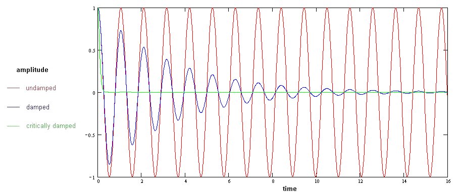
The frequency varies as the square root of the ratio of two quantities (i) the elasticity or degree of stability (in this case the 'stiffness' of the spring K), and (ii) a coefficient of inertia (in this case the 'inertial mass' m). To produce mechanical waves, a system must have the means of storing potential energy (for example, in a spring) and kinetic energy (for which there must 'inertial mass' which can be 'localised' or 'distributed'). As we saw with the simple pendulum, undamped vibratory motion is associated with the transformation of potential to kinetic energy, or the reverse, while the sum of these two forms of energy remains constant. If the system is damped, and energy is steadily lost to some damping mechanism (generally through frictional forces, for example, air resistance), the system may continue its vibratory motion but with a steadily reducing amplitude.
A mass m, attached to a horizontal massless spring with spring constant K, free to move on a horizontal frictionless surface, also exhibits SHM.
In this case, because the force due to gravity acting on the mass is perpendicular to the direction of the spring, the equilibrium position of the system as a whole is that where the spring is stretched to its natural length, i.e. the greatest length where the spring generates no force.
Some authors use 'compliance' C in place of 'stiffness' K where C = 1 / K. In this caseωo2 = (1 / Cm).
Free Oscillations - Spring of Air
A piston is free to move in a vertical cylinder above a volume of air trapped below it. As the piston moves to compress the air below it, a force acting against the motion acts like a spring. In its equilibrium position, the piston slightly compresses the gas in the cylinder to balance the gravitational force due to the mass of the piston. The problem turns out to be no more than finding the correct expression for the 'spring constant' of the air.
Let m be the mass of the piston, L and S the length and surface cross-sectional area of of the cylinder, pa the atmospheric pressure and γ the ratio of the specific heats of air. The relationship for adiabatic compression between the pressure in the cylinder pi and the volume of air in the cylinder Vi, which from simple geometry equals SL, is
pi Viγ = a constant.
The differential equation for the motion of the piston is
| d 2x | = | S dpi |
| dt 2 | m |
where dpi is the increase in the air pressure in the cylinder, above that when the piston is in its equilibrium position, acting against the piston when, moving a distance x downwards from its equilibrium position, it compresses the air in the cylinder. Downward motion is associated with x increasingly negative and pi increasingly positive.
dpi = -pa γ x / L
from which
| = | 1 | γpaS | ||
| fo | ||||
| 2π | mL |
The Action of Frictional Forces
Friction between solid bodies (called 'sliding friction') is usually independent of their relative velocity. However, a particle moving through a fluid (a gas or a liquid) experiences frictional forces, (e.g. internal damping saps energy from the oscillator and converts it into heat), that are generally proportional to the speed and act to oppose the motion. Let us re-examine the dynamics of a mass attached to a massless spring moving horiontally in the presence of a frictional force of this kind.
| m | d 2x dt 2 | + R | dx dt | + K x | = 0 |
Using methods developed by Euler and d'Alembert, we try a complex solution of the form x = A exp ( j φ ) exp ( λ t ), where x is the complex displacement and A exp ( j φ ) is the complex amplitude. We find that
( λ 2 + 2 ( R / 2m) λ + ( K / m ) 2 ) A exp ( j φ ) exp ( λ t ) = 0.
K / m = ω o , the natural angular frequency in the absence of any damping force.
The left-hand term, on the left-hand side of the equation, is quadratic and there are two possible values for λ.
If ω d is the natural angular frequency of the damped oscillator, where ω d 2 = ω o 2 - (R / 2m ) 2 , the general solution is:
x = exp ( - Rt / 2m ) { A1 exp ( j φ ) exp ( j ω d t ) + A2 exp ( - j φ ) exp ( - j ω d t ) }
The real displacement Re [ x ], found by taking the real part of the general solution above, is
x = A exp ( - Rt / 2m ) cos ( ω d t + φ )
The presence of the exponential term in the solution means that the behaviour is not strictly periodic although the system passes periodically through its equilibrium position x = 0 because where the amplitude is zero, that value remains the same. That period T d = 2 π / ω d.
In addition, one can characterise the decay in the amplitude, say the time to reduce the amplitude to 1 / e of its initial value, with a term called decay time, relaxation time or modulus of decay τ = 2m / R
It is worth mentioning that frictional decay in acoustics is generally a slow process.
In such cases, ω d 2 > 0.
If however, ω d 2 = 0 the system is said to be 'critically' damped and the real displacement is given by:
x c = x o ( 1 + ( Rt / 2m ) ) exp ( - Rt / 2m ).
If ω d 2 < 0 the system is said to be overdamped and the system slowly decays passing at most once through its zero position. This behaviour is also called 'dead-beat'.
Forced Oscillations
If our simple oscillator is driven by an external force f (t), the equation of motion is
| m | d 2x dt 2 | + R | dx dt | + K x | = f (t) |
The external force f (t) may be impulsive, periodic or non-periodic. Of particular interest is a driving force that is periodic and starts at a particular time. We wish to investigate the behaviour of the system from when the force is applied.
Although the solution consists of two parts, we will consider the transient behaviour later. Let us consider first the steady-state behaviour. Let f (t) = F exp ( j ω t ) where the force function is in its complex form.
The linearity of the equation leads us to expect, that in the steady state, both sides of the equation should be harmonic with the same frequency. Replacing the complex variable x by A exp ( j φ ) exp ( j ω t ),
| A exp ( j φ ) exp ( j ω t ) = x = | F exp ( j ω t ) ( - ω 2 m + j ω R + K ) |
Substituting ω o 2 for K / m and α for R / 2m the equation can be rewritten
| x = | ( F / m ) exp ( j ω t ) ( ω o 2 - ω 2 + j ω 2 α ) |
The real part of this equation, the steady-state displacement, is given by
| x = | F sin ( ω t + φ ) ω Z |
where Z = R + j ( ω m - K / ω ) = R + j X m .
Z is the mechanical impedance and X m is the mechanical reactance.
If ω is very small, the real value of x reduces to F / K . In effect we are looking at a situation where the oscillator has been displaced by a constant force, a region where the oscillator is said to be stiffness dominated. This value of x , written x s , is defined as the static displacement.
If ω = ω o , the maximum value for the displacement x max = F / ω o R .
One particular feature of the system when the value of ω is close to ω o is the shape of the curve that describes the value of x / x s versus ω / ω o.
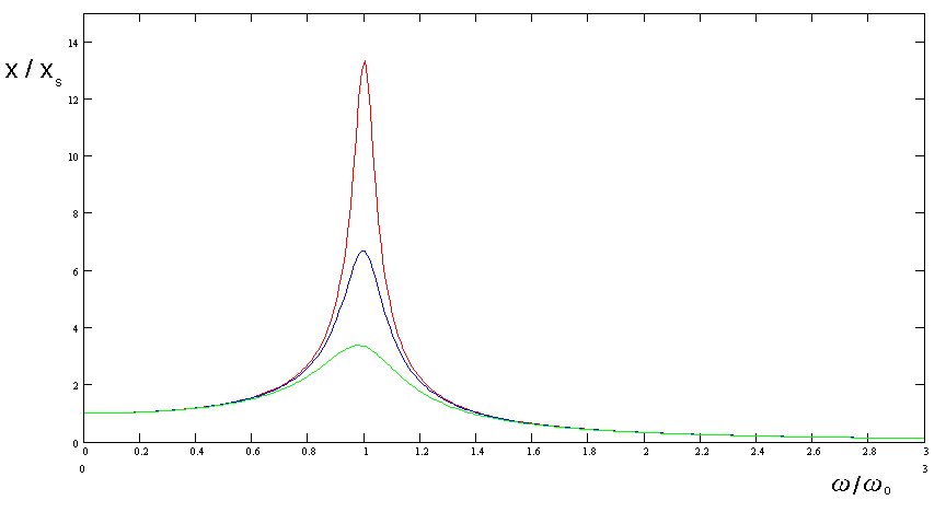
The peak of this curve, 'the resonance peak', becomes wider and higher as the frictional force R increases. This is why the region is described as 'resistance' dominated. Some characterise the sharpness of the curve by the ratio of ω to the full width of the peak at one half the maximum height Δ ω .
When ω = ω o , the system is said to be at resonance. The amplification factor Q is defined as the ratio of maximum amplitude at resonance x max to the static displacement x s .
Q = x max / x s = K / ω o R
This relationship explains why, by imparting energy at exactly the right point in the motion of an oscillator, the amplitude of oscillation can be increased, something even small children discover when playing on a garden swing. If there is little or no damping, the amplitude of oscillation associated with resonance can get very large, as, for example, when the Tacoma suspension bridge collapsed or when the Millennium footbridge over the river Thames in London began to move alarmingly as large numbers of people were walking across it. In the case of the footbridge over the Thames, engineers fitted large mechanical damping devices to the bridge to restrict its motion to acceptable limits. There are examples of resonance in every area of physics as Richard Feynman so delightfully points out in section 23-4 of book 1 of his Lectures on Physics to which anyone interested in this topic is recommended to turn. |
When ω >> ω o , i.e. the frequency of the external force is much greater than the natural frequency of the system undergoing free oscillation, the displacement falls to zero and the system is described as being mass dominated.
The ratio x o / x is less than unity where ω 2 > ( 2 ω o2 - ( R / m ) 2 )
One can also examine the phase angle between the displacement and the driving force for different frequencies.
| φ x - φ F = | tan -1 | - R ω / m ω o2 - ω 2 |
Because tan ( - θ ) = - tan ( θ ) we see that the displacement lags behind the driving force.
When ω << ω o the phase shift tends to 0° ; when ω = ω o the phase shift is 90° ( π / 2 radians ); and when ω >> ω o the phase shift tends towards 180° ( π radians).
The frequency response of a simple oscillator can be 'described' in many ways, each providing its own 'physical' insight. For example, one might consider how the mechanical impedance or its reciprocal, the mechanical admittance (or mobility), varies with frequency. These are complex quantities and we need to consider the behaviour both of their real and imaginary parts.
To the physicist, resonance plays an important role in the way energy is absorbed by a system. At resonance, the system needs a lot of energy in order to increase its amplitude of motion. Outside that region, when the amplification is equal to or less than 1, the energy drawn from the external source will be relatively small. Put another way, the system has an increased capacity for absorbing energy when it is close to resonance but only a relatively small capacity when far away from resonance. Absorption peaks, observed when light passes through matter, correspond with frequencies for which elements of the system are at or are close to resonance (see: Lorentz's Theory of Dispersion in Dielectrics). |
Let us now briefly mention the other part of our solution, which describes the transient behaviour at and shortly after the application of the driving force. As the system moves from its steady state free oscillation to its new steady state, analysis of its behaviour can be involved. The time scale of its intermediate behaviour depends on a number of parameters, particularly, the degree of damping in the system. A heavily damped system reaches its new steady state quickly because any transient behaviour decays rapidly. When damping is light, transient behaviour is prolonged. If the driving and natural frequencies are close, the system can exhibit 'beating' with a frequency equal to the difference between the two frequencies. In every case, the system will, after some time, find its new steady-state behaviour.
The linearity of the equation
| m | d 2x dt 2 | + R | dx dt | + K x | = f (t) |
leads us to expect a general solution that combines the solution for a free damped oscillator (the homogeneous equation) and the steady state solution for an oscillator undergoing forced oscillation (the particular solution).
Our main task would be to choose suitable values for the initial conditions which determine the values of the arbitrary constants A and φ.
